This post is a follow-up to the previous one in which we explored the problem of ACL tears and the related MRNet dataset released by Stanford ML group. If you want to learn more about Stanford's work you can visit this link.
Today, we are going to use MRNet data to build a Convolutional Neural Network that detects and classifies ACL tears from MRI scans. We will implement it in PyTorch to fully take advantage of the capabilities of this framework.
By the end of this post you will learn a few things:
- How to write a convolutional neural network specifically designed to process MRI scans for a given plane (axial,sagittal and coronal): we will see that this architecture slightly differs from conventional cnn architectures that classify natural images
- How to implement a "meta-model" that combines the predictions of the aforementioned cnn models trained individually to classify ACL injury on each plane
- How to handle the lack of MRI data using transfer learning and data augmentation
- How to build an end to end PyTorch training pipeline to load and process data, train, monitor and evaluate the models
If you reach the end of this article, you should have a global overview of the ACL tear classification problem.
Note: if this medical task doesn’t interest you in particular, you can reuse some blocks for other medical imaging tasks such as tumor classification.
Reminder of the problem
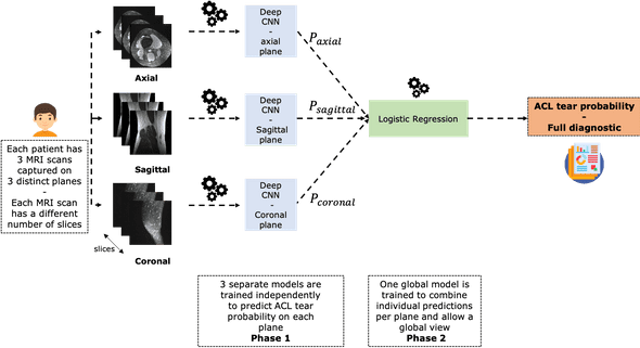
This chart summarizes the problem and the way we're going to address it:

As you can see it, each patient has three MRI scans taken with respect to three different planes: axial, sagittal and coronal.
We are going to build 3 independent CNN models that allow to classify ACL tear per plane.
Each of these networks will specialize in detecting ACL tear from a given plane. In order to have a model that performs well everywhere, we will combine these three models using a stacking operation.
In practice, we are going to train a logistic regression on the CNNs probability outputs to predict ACL tear.
This is an important step that is supposed to mimic the way radiologists consider different MRI scans (in different planes) of a single patient in order to make a robust diagnostic.
MRNet architecture
Let's now detail the CNN model architecture that will be common to the three networks. The Stanford team named it the MRNet.
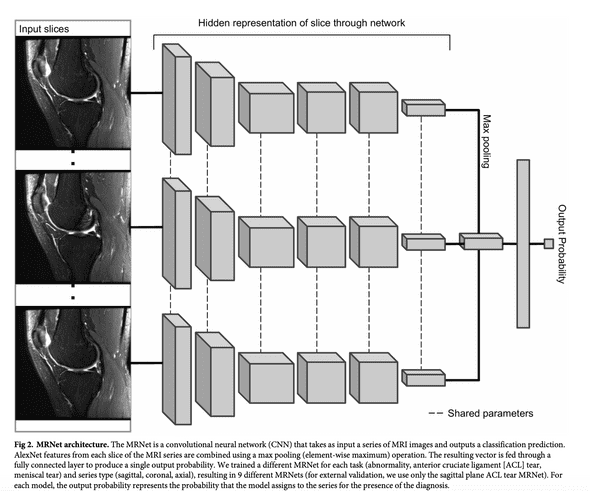
The MRNet is a convolutional neural network that takes as input an MRI scan and outputs a classification prediction, namely an ACL tear probability.
The input has dimensions s x 3 x 256 x 256 where s is the number of slices (i.e. images) in the MRI scan. 3 is number of color channel per slice.
First, each MRI slice is passed through a feature extractor based on a pre-trained AlexNet to obtain a s x 256 x 7 x 7 tensor containing features for each slice. A global average pooling layer is then applied to reduce these features to s x 256. Basically, each 7x7 matrix is reduced to its mean.
Then max pooling across slices is applied to obtain a 256-dimensional vector which is passed a fully connected layer and sigmoid activation function to obtain a prediction between 0 an 1.
The chart below, taken from Stanford's paper, illustrates this architecture.

Some points to notice about this architecture:
- Given that s varies from a patient to another, it is impossible to stack piles of MRI in batches. Therefore, we will use batches of size 1 during training
- Slices are fed in parallel in AlexNet the same way batches of natural images are processed in parallel by this pretrained network
Training procedure
The training of the model is done through the minimization of the cross-entropy loss using Adam optimizer.
To take into account the imbalanced nature of the classes, the loss of an example was scaled inversely proportionally to the prevalence of that example’s class in the dataset in order to penalize the error more on the least present examples.
During training, the gradient of the loss is computed on each training example using the backpropagation agorithm and the network's parameters are then adjusted in the opposite direction of the gradient.
During training, some geometric transformations are applied on the input MRI. These transformations are label-invariant. They are meant to bring diversity in the dataset and increase the stability of the model while decrease its tendency to overfitting. This procedure is called data augmentation.
We'll sequentially apply 3 geometric transformations on each input MRI.
- Random rotation between -25 and 25 degrees
- Random shift in both direction between -25 and 25 pixels
- Random horizontal flip with 50% probability
Note that data augmentation is done identically over all the slices of an MRI.
Code structure
Let's now turn what we've just seen into a PyTorch implementation.
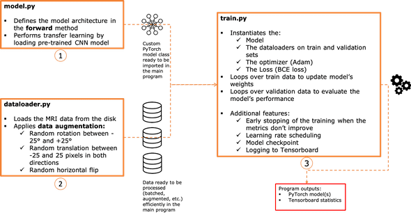
We will organize the source code in three main files (all the code available on github ):
- model.py
- dataloader.py
- train.py
The chart below summarizes pretty much the responsibility of each script.

1 - The model architecture: model.py
import torch
import torch.nn as nn
from torchvision import models

class MRNet(nn.Module):
    def __init__(self):
        super().__init__()
        self.pretrained_model = models.alexnet(pretrained=True)
        self.pooling_layer = nn.AdaptiveAvgPool2d(1)
        self.classifer = nn.Linear(256, 1)

    def forward(self, x):
        x = torch.squeeze(x, dim=0)
        features = self.pretrained_model.features(x)
        pooled_features = self.pooling_layer(features)
        pooled_features = pooled_features.view(pooled_features.size(0), -1)
        flattened_features = torch.max(pooled_features, 0, keepdim=True)[0]
        output = self.classifer(flattened_features)
        return output
This model is actually quite simple. We define it as a class called MRNet that inherits from the torch.nn.Module class.
In the constructor we define three objects:
- the pretrained AlexNet model
- the pooling layer
- the dense layer that acts as a classification layer
In the forward method, we actually write the forward pass, i.e. the operations the network performs on the input until it computes the predictions.
Let's detail it step by step:
- this method recieves an input x of shape (1, s, 256, 256, 3) since, as we said earlier, we are dealing with batches of size 1
- it removes the first dimension by "squeezing" the input and turning its shape to (s, 256, 256, 3)
- now (s, 256, 256, 3) is a regular tensor shape that can be fed to an AlexNet which produces the features of shape (s, 256, 7, 7) afterwards
- the features are pooled which produces an output of shape (s, 256)
- the pooled features are flattened in a 256 dimension vector that is finally fed to the classifier that outputs a scalar value. Note that we don't use a sigmoid activation here. Sigmoid is applied in the loss direction.
2 - The custom dataset: dataloader.py
In this script, we define a custom Dataset object that loads the MRNet data in the main program.
To create the dataset, we define a class called MRDataset that inherits from the class torch.utils.data.Dataset
class MRDataset(data.Dataset):
    def __init__(self, root_dir, task, plane, train=True, transform=None, weights=None):
        super().__init__()
        self.task = task
        self.plane = plane
        self.root_dir = root_dir
        self.train = train
        if self.train:
            self.folder_path = self.root_dir + 'train/{0}/'.format(plane)
            self.records = pd.read_csv(
                self.root_dir + 'train-{0}.csv'.format(task), header=None, names=['id', 'label'])
        else:
            transform = None
            self.folder_path = self.root_dir + 'valid/{0}/'.format(plane)
            self.records = pd.read_csv(
                self.root_dir + 'valid-{0}.csv'.format(task), header=None, names=['id', 'label'])

        self.records['id'] = self.records['id'].map(
            lambda i: '0' * (4 - len(str(i))) + str(i))
        self.paths = [self.folder_path + filename +
                      '.npy' for filename in self.records['id'].tolist()]
        self.labels = self.records['label'].tolist()

        self.transform = transform
        if weights is None:
            pos = np.sum(self.labels)
            neg = len(self.labels) - pos
            self.weights = [1, neg / pos]
        else:
            self.weights = weights

    def __len__(self):
        return len(self.paths)

    def __getitem__(self, index):
        array = np.load(self.paths[index])
        label = self.labels[index]
        label = torch.FloatTensor([label])

        if self.transform:
            array = self.transform(array)
        else:
            array = np.stack((array,)*3, axis=1)
            array = torch.FloatTensor(array)

        if label.item() == 1:
            weight = np.array([self.weights[1]])
            weight = torch.FloatTensor(weight)
        else:
            weight = np.array([self.weights[0]])
            weight = torch.FloatTensor(weight)

        return array, label, weight
In the constructor of MRDataset, we define a set of arguments:
- root_dir: ./data/
- task: either acl, meniscus or abnormal. we'll focus on acl in this post
- plane: either sagittal, coronal or axial
- train: a boolean variable that indicates whether we are processing train data or not (validation)
- transform: the series of data augmentation operations. If None, no data augmentation
- weights: custom weights for each class (default to None): this is used to adjust the loss function. When None, weights are computed automatically.
In the remaining part of the constructor, we prepare the paths, the labels, and the weights that correspond to each data sample.
In the __len__ function, we return the length of the data
In the __getitem__ function we return the MRI scan .npy file, the label and the weight after applying minor preprocessing and eventual data augmentation.
3 - Where the training happens: train.py
This script is the main part of the application. It does the heavy lifting and outputs (i.e. saves) a trained model.
Here is what it does in a nutshell:
- It imports dataloader.py to load the data from both train or validation sets.
- It imports model.py and instantiates an MRNet model before updating its weights.
- It launches a training and validation loop over a given number of epochs.
If we skip everything and look at the first line of code that is executed when the script is called from terminal,
if __name__ == "__main__":
    args = parse_arguments()
    run(args)
... we'll see that it starts by loading some arguments that are given in the command line.
def parse_arguments():
    parser = argparse.ArgumentParser()
    parser.add_argument('-t', '--task', type=str, required=True,
                        choices=['abnormal', 'acl', 'meniscus'])
    parser.add_argument('-p', '--plane', type=str, required=True,
                        choices=['sagittal', 'coronal', 'axial'])
    parser.add_argument('--augment', type=int, choices=[0, 1], default=1)
    parser.add_argument('--lr_scheduler', type=int, choices=[0, 1], default=1)
    parser.add_argument('--epochs', type=int, default=50)
    parser.add_argument('--lr', type=float, default=1e-5)
    parser.add_argument('--flush_history', type=int, choices=[0, 1], default=0)
    parser.add_argument('--save_model', type=int, choices=[0, 1], default=1)
    parser.add_argument('--patience', type=int, choices=[0, 1], default=5)

    args = parser.parse_args()
    return args
Once the arguments are loaded in the args variable, the run function starts executing.
Without going into much details, this function first starts by creating a folder that'll be used by tensorboard to save the training logs and visualize the metrics of the training session:
On each run of the script, a new folder (named after the timestamp) is created:
def run(args):
    log_root_folder = "./logs/{0}/{1}/".format(args.task, args.plane)
    if args.flush_history == 1:
        objects = os.listdir(log_root_folder)
        for f in objects:
            if os.path.isdir(log_root_folder + f):
                shutil.rmtree(log_root_folder + f)

    now = datetime.now()
    logdir = log_root_folder + now.strftime("%Y%m%d-%H%M%S") + "/"
    os.makedirs(logdir)

    writer = SummaryWriter(logdir)
Then we define the data augmentation pipeline
    # data augmentation pipeline
    augmentor = Compose([
        transforms.Lambda(lambda x: torch.Tensor(x)),
        RandomRotate(25),
        RandomTranslate([0.11, 0.11]),
        RandomFlip(),
        transforms.Lambda(lambda x: x.repeat(3, 1, 1, 1).permute(1, 0, 2, 3)),
    ])
and instantiate a train and validation MRDataset(s).
    train_dataset = MRDataset('./data/', args.task, args.plane, transform=augmentor, train=True)
    validation_dataset = MRDataset('./data/', args.task, args.plane, train=False)
These datasets are now passed to a Dataloader which is a handy PyTorch object that allows to efficiently iterate over the data by leveraging batching, shuffling, multiprocessing and data augmentation.
    train_loader = torch.utils.data.DataLoader(
        train_dataset, batch_size=1, shuffle=True, num_workers=11, drop_last=False)

    validation_loader = torch.utils.data.DataLoader(
        validation_dataset, batch_size=1, shuffle=-True, num_workers=11, drop_last=False)
Now we instantiate the MRNet model and pass its paramaters to GPU.
We define the Adam optimizer as well as a learning rate scheduler.
We instantiate the number of epochs and the patience i.e. the minimum number of epochs without improvement of the loss.
    mrnet = model.MRNet()
    mrnet = mrnet.cuda()

    optimizer = optim.Adam(mrnet.parameters(), lr=1e-5, weight_decay=0.1)
    scheduler = torch.optim.lr_scheduler.ReduceLROnPlateau(
        optimizer, patience=3, factor=.3, threshold=1e-4, verbose=True)

    best_val_loss = float('inf')
    best_val_auc = float(0)

    num_epochs = args.epochs
    iteration_change_loss = 0
    patience = args.patience
Now comes the best part, the training part:
    for epoch in range(num_epochs):

        train_loss, train_auc = train_model(
            mrnet, train_loader, epoch, num_epochs, optimizer, writer)
        val_loss, val_auc = evaluate_model(
            mrnet, validation_loader, epoch, num_epochs, writer)

        print("train loss : {0} | train auc {1} | val loss {2} | val auc {3}".format(
            train_loss, train_auc, val_loss, val_auc))

        if args.lr_scheduler == 1:
            scheduler.step(val_loss)

        iteration_change_loss += 1
        print('-' * 30)

        if val_auc > best_val_auc:
            best_val_auc = val_auc
            if bool(args.save_model):
                file_name = f'model_{args.task}_{args.plane}_val_auc_\
                            {val_auc:0.4f}_train_auc_{train_auc:0.4f}\
                            _epoch_{epoch+1}.pth'
                for f in os.listdir('./models/'):
                    if (args.task in f) and (args.plane in f):
                        os.remove(f'./models/{f}')
                torch.save(mrnet, f'./models/{file_name}')

        if val_loss < best_val_loss:
            best_val_loss = val_loss
            iteration_change_loss = 0

        if iteration_change_loss == patience:
            print('Early stopping after {0} iterations without the decrease of the val loss'.
                  format(iteration_change_loss))
            break
On each epoch, many things are executed:
- We train the model using train_model
- We evaluate the model using evaluate_model
- We print the AUC metric and the loss on train and validation data
- We let the learning rate scheduler update the learning rate
- if the validation AUC improves we checkpoint the model to disk
- if the number of epochs without improvement of the loss is higher than the patience, we interrupt the training
Let's now focus on the train_model function that is called on each epoch.
Here's the full code:
def train_model(model, train_loader, epoch, num_epochs, optimizer, writer, log_every=100):
    _ = model.train()
    if torch.cuda.is_available():
        model.cuda()
    y_preds = []
    y_trues = []
    losses = []

    for i, (image, label, weight) in enumerate(train_loader):
        optimizer.zero_grad()

        if torch.cuda.is_available():
            image = image.cuda()
            label = label.cuda()
            weight = weight.cuda()

        prediction = model.forward(image.float())

        loss = F.binary_cross_entropy_with_logits(
            prediction[0], label[0], weight=weight[0])

        loss.backward()
        optimizer.step()

        y_pred = torch.sigmoid(prediction).item()
        y_true = int(label.item())

        y_preds.append(y_pred)
        y_trues.append(y_true)

        try:
            auc = metrics.roc_auc_score(y_trues, y_preds)
        except:
            auc = 0.5

        loss_value = loss.item()
        losses.append(loss_value)

        writer.add_scalar('Train/Loss', loss_value,
                          epoch * len(train_loader) + i)
        writer.add_scalar('Train/AUC', auc, epoch * len(train_loader) + i)

        if (i % log_every == 0) & (i > 0):
            print('''[Epoch: {0} / {1} |Single batch number : {2} / {3} ]\
                    | avg train loss {4} | train auc : {5}'''.
                  format(
                      epoch + 1,
                      num_epochs,
                      i,
                      len(train_loader),
                      np.round(np.mean(losses), 4),
                      np.round(auc, 4)
                  )
                  )
    writer.add_scalar('Train/AUC_epoch', auc, epoch + i)
    train_loss_epoch = np.round(np.mean(losses), 4)
    train_auc_epoch = np.round(auc, 4)
    return train_loss_epoch, train_auc_epoch
Let's break it into pieces:
We start by setting the model to train mode, then pass it to GPU and initialize the lists that will contain predictions, true labels and the losses on each individual sample.
    _ = model.train()
    if torch.cuda.is_available():
        model.cuda()
    y_preds = []
    y_trues = []
    losses = []
Then we loop over the dataloader:
At each step:
- A single MRI scan and its corresponding label and weight are passed to GPU
- The network computes a forward pass on the MRI scan which results in a prediciton
- The loss between the prediction and the true label is computed
- Backpropagation of the loss: computation of the gradients
- Weights update by the optimizer
    for i, (image, label, weight) in enumerate(train_loader):
        optimizer.zero_grad()

        if torch.cuda.is_available():
            image = image.cuda()
            label = label.cuda()
            weight = weight.cuda()

        loss = F.binary_cross_entropy_with_logits(
            prediction[0], label[0], weight=weight[0])

        loss.backward()
        optimizer.step()
The remaining code executed on each epoch monitors the training metrics and logs them to Tensorboard.
Results: classification of ACL tears on sagittal plane
- Setup: Nvidia 1080 Ti and i7 8700K CPU.
- Training took approximately 1h and 11 minutes. 35 epochs.
-
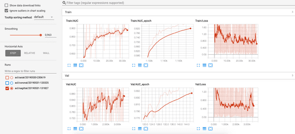
The best model is saved on disk with the following AUC scores
- On train set: 0.8669
- On validation set: 0.8850
The AUC and the loss can be viewed in Tensorboard at each epoch and each batch:

Building a global ACL tear classifer
Now that we've seen how to train an ACL tear classifier on the sagittal plane, we can follow the same procedure for the two other planes. Results are comparable.
When the three models and trained and saved to disk, we use them to compute predictions on each sample of training and validation.
def extract_predictions(task, plane, train=True):
    assert task in ['acl', 'meniscus', 'abnormal']
    assert plane in ['axial', 'coronal', 'sagittal']

    models = os.listdir('../models/')

    model_name = list(filter(lambda name: task in name and plane in name, models))[0]
    model_path = f'../models/{model_name}'

    mrnet = torch.load(model_path)
    _ = mrnet.eval()

    train_dataset = MRDataset('../data/',
                              task,
                              plane,
                              transform=None,
                              train=train,
                              normalize=False)

    train_loader = torch.utils.data.DataLoader(train_dataset,
                                               batch_size=1,
                                               shuffle=False,
                                               num_workers=10,
                                               drop_last=False)
    predictions = []
    labels = []
    with torch.no_grad():
        for image, label, _ in tqdm_notebook(train_loader):
            logit = mrnet(image.cuda())
            prediction = torch.sigmoid(logit)
            predictions.append(prediction.item())
            labels.append(label.item())

    return predictions, labels
The predictions computed on train data become new features for training a logistic regression.
task = 'acl'
results = {}

for plane in ['axial', 'coronal', 'sagittal']:
    predictions, labels = extract_predictions(task, plane)
    results['labels'] = labels
    results[plane] = predictions

X = np.zeros((len(predictions), 3))
X[:, 0] = results['axial']
X[:, 1] = results['coronal']
X[:, 2] = results['sagittal']

y = np.array(labels)

logreg = LogisticRegression(solver='lbfgs')
logreg.fit(X, y)
Once the logistic regression is trained, we evaluate it on the validation features i.e the models' predictions on validation data.
task = 'acl'
results_val = {}

for plane in ['axial', 'coronal', 'sagittal']:
    predictions, labels = extract_predictions(task, plane, train=False)
    results_val['labels'] = labels
    results_val[plane] = predictions

y_pred = logreg.predict_proba(X_val)[:, 1]
metrics.roc_auc_score(y_val, y_pred)
Result: we get an AUC of 0.95
Wrap-up: where to go from here?
You just learnt about ACL tear classification using a deep convolutional neural network.
Now is time to check what this model actually learnt. In the next post, we'll investigate an interpretation method that highlights image areas that activate in case of an ACL tear. We'll use this method as a support for validation and augmented diagnosis. It's also a helpful tool that allow radiologists trust machine learning models.