This post is the third and last one of a series I dedicated to medical imaging and deep learning. If you're interested in this topic you can read my first article where I explore the MRNet knee MRI dataset released by Stanford and my second article where I train a convolutional neural network to classify the related knee injuries. The model is implemented in PyTorch and the source code is now available on my github repo.
In this post, we will focus on interpretability to assess what the model(s) we trained actually learnt from the MRI scans so that its (their) predictions can be explained to a real radiologist. The goal of this tutorial is to get you familiar with a popular interpretability technique called Class Activation Map, applied when using convolutional neural networks that have a special architecture.
This will hopefully give you more confidence in your models’ predictions and provide you with the ability to better explain them to a larger audience.
Throughout this post, we'll be covering the following topics:
- Model interpretability and the importance of explaining complex decisions in sensitive application areas
- How to make Convolutional Neural networks interpretable by visualizing their predictions through the Class Activation Map (CAM)
- How to implement this method in PyTorch
Class Activation Map is a method that is completely generic and can be reproduced and applied to different computer vision projets. So feel free to play with the code and adapt it to meet your needs.
Machine learning and the urge of interpretability

Model interpretability encompasses the different tools and techniques that allow to inspect and understand why a predictive model provided a given prediction to a given input.
With machine learning models being more and more deployed to production environments in various sectors such as financial services, defense and healthcare, the ability to answer this question becomes critical. In fact, having a machine learning model with good performance metrics is barely enough for today's business purposes. What the industry needs is knowing the decision process behind each decision to motivate further actions.
Here are some examples of real-world scenarios I came accross in my experience and where I think interpretability matters:
- If you're building a credit scoring engine that denies a credit application to a customer, you are legally obliged to provide a comprehensive justification based on the variables that were used in the computations and led to the credit denial
- When working on fraud detection either for insurance or financial services, you must motivate to the business why you suspect a fraud and why your model should be trusted. In fact, the business will not take your output for granted. They'll have to inspect the causes and the features that highlighted the suspicious behavior before taking any investigation steps that could take time and resources at different levels of the organization.
- When designing a job recommendation engine to help human resources managers, you have to make sure that your models are not biased toward specific attributes such as the gender, the age or the ethnicity.
We could think of a lot more reasons to introduce interpretability. Today's focus, as you expect it, is healthcare.
The question we'll try to answer is the following:
What makes the Convolutional Neural Network MRNet model we trained think a given patient is subject to an ACL tear by "looking" at his MRI exam?
The problem with Convolutional Neural Networks
Convolutional Neural Networks have a special architecture that allows them to represent images in a way classification problems become a lot easier. This is done by converting the input into a feature vector that is supposed to condense all the important visual informations that were initially present in the image. If you're building a car classifier for example, you could think of one of these features as the presence (or the absence) of wheels.
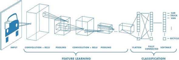
If you're interested in learning more about ConvNets; how they work and how to use them in practical use cases, I encourage you to go through a post I wrote on this topic about one year ago.
Although ConvNets have became very efficient lately by outperforming the human eye in visual tasks of different levels of complexitiy, one question still arises a lot: are we able to explain why these networks work so well?
There are two ways to answer this question.
If you're interested in the theory behind these networks, you can dive into pure mathematical considerations and watch Stéphane Mallat's excellent presentation in which he approaches and explains ConvNets in a mathematical formalism by introducing his famous theory of wavelets.
The other way to build an intuition on why ConvNets work is by visualizing the salient areas these networks focus on before making a prediction when confronted with an image.
Just like humans rapidly recognize objects by focusing on their important visual attributes (the wings for birds or the trunk for elephants), ConvNets virtually do the same by attending to some regions.
By "going backward" in the network, some techniques allow to highlight the image regions that were most activated for a given class. There's of course a lot of techniques. Today, we'll be looking at a popular one called Class Activation Map and introduced in this paper.
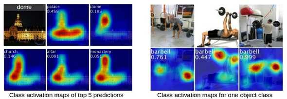
Reminder on the Global Average Pooling layer
This layer is an important block of your network if you want to use Class Activation Map. Without it, computing CAM is not possible.
This layer is used in MRNet after the last convolutional layer of the AlexNet pretrained network.
What it does is actually pretty simple: when confronted with a number (depth) of filters of size (height x width), it reduces each one to its spatial mean. In other terms, it performs independant average poolings over each filter and stack the results in a vector of size 1 x 1 x depth.
We'll see it next; filters with high activations will hive higher signal.
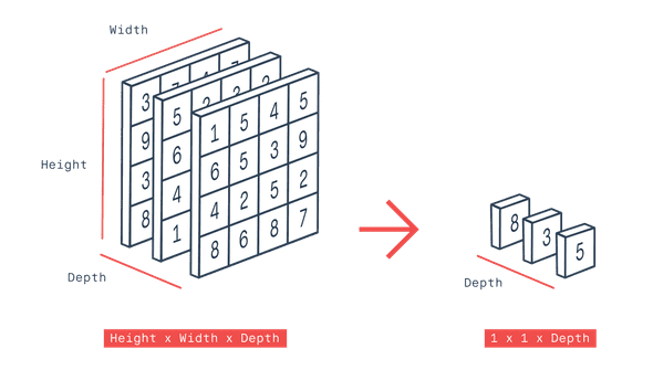
Class Activation Map
Class Activation Map (CAM) is a technique that allows to highlight discriminative regions used by a CNN to indentify a class in the image.
As we stated before, to be able to build a CAM, the CNN must have a global average pooling layer after the final convolutional layer and then a linear (dense) classification layer. This means that this method cannot unfortunately be directly applied to all CNN architectures. The trick is to plug an existing pretrained network to a global average pooling layer and then finetune this layer through additional training.
CAM is still powerful and easy to put in place. Let's now see how it's generated for a simple 2D image.
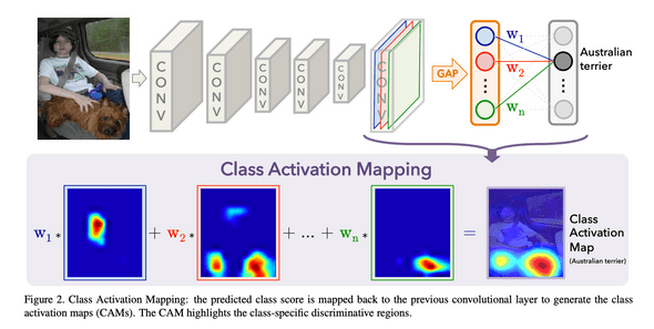
When fed with a 2D color image, a CNN constrained with a global average pooling layer, outputs after the last convolutional layer a set of filters (blue, red ... green in figure above) that get redued to a vector after global average pooling. This vector is then connected to a final classification layer to output the predicted class.
- Each filter (blue, red, ... green), contains a 2D low-level spatial information about the image that got distilled after layers of successive convolutions.
- Each weight w1, w2, ... wn represent the partial importance of each reduced filter in determining the output class (Australian terrier).
These filters and weights adjust throughout training by the back-propagation algorithm.
The author of the paper defined class activation map as a weighted sum of the filters by the weights w1, w2, ... wn
A Class Activation Map is therefore a sum of a set of spatial 2D activations (i.e filters) weighted with respect to their relative importance in determining the output class.
When a class activation map is generated, it obviously has not the dimension of the initial image (it has the dimension of filters of the last conv layer). To be able to use it and superpose it to the input, an upsampling opreation is done to resize it.
When superposed to the initial image, CAM is represented as a heatmap in which discriminative regions are painted in red.
CAM implementation in PyTorch
Let's start by generating CAMs for simple classes from the ImageNet dataset. To do this, we'll be using pretrained networks that have a Global Average Pooling layer.
Hopefully, some of these networks are available in torchvision:
- squeezenet1_1
- resnet18
- densenet161
We'll be using: resnet18
from IPython.core.display import display,HTML
display(HTML('<style>.prompt{width: 0px; min-width: 0px; visibility: collapse}</style>'))

%matplotlib inline
%config Completer.use_jedi=False

import os
import io
import requests
from PIL import Image
from torchvision import models, transforms
from torch.autograd import Variable
from torch.nn import functional as F
import numpy as np
import cv2
import pdb

from matplotlib import pyplot as plt

model_id = 2
if model_id == 1:
    net = models.squeezenet1_1(pretrained=True)
    finalconv_name = 'features' # this is the last conv layer of the network
elif model_id == 2:
    net = models.resnet18(pretrained=True)
    finalconv_name = 'layer4'
elif model_id == 3:
    net = models.densenet161(pretrained=True)
    finalconv_name = 'features'
Once the model is loaded, we have to define a function that extracts the result of the final convolution layer once a image goes through the network in a forward pass.
Since PyTorch doesn't allow to access this result directly, we'll have to wrap this function inside the registerforwardhook method. This means that the output will be extracted each time the network makes a forward pass.
net.eval()

# hook the feature extractor
features_blobs = []
def hook_feature(module, input, output):
    features_blobs.append(output.data.cpu().numpy())

net._modules.get(finalconv_name).register_forward_hook(hook_feature);
Now we extract the weights connecting the output of the class activation map (the vector in orange) to the final (classification) layer
params = list(net.parameters())
weight_softmax = np.squeeze(params[-2].data.numpy())
This tensor has the shape : (1000, 512). It connects 512 reduced filters to 1000 output classes.
Now let's define a function that computes a CAM for a given image.
Assuming this function has the following arguments:
- feature_conv: the output of the last conv layer after passing the image through the network
- weight_softmax: the weights connecting the output of the class activation map to final (classification) layer
- class_idx: the index(es) of the predicted class(es)
it'll for each class:
- compute the class activation map as a dot product between the weights and the filters and store it in the variable
cam - normalize
cam - upsample it to original size (256, 256)
def returnCAM(feature_conv, weight_softmax, class_idx):
    # generate the class activation maps upsample to 256x256
    size_upsample = (256, 256)
    bz, nc, h, w = feature_conv.shape
    output_cam = []
    for idx in class_idx:
        cam = weight_softmax[idx].dot(feature_conv.reshape((nc, h*w)))
        cam = cam.reshape(h, w)
        cam = cam - np.min(cam)
        cam_img = cam / np.max(cam)
        cam_img = np.uint8(255 * cam_img)
        output_cam.append(cv2.resize(cam_img, size_upsample))
    return output_cam
Let's donwload this image from the internet and extract possibles CAMs out of it:

We first apply a series of normalization steps to the image.
We then pass it through the network, get the top classes and their respective probabilities.
normalize = transforms.Normalize(
   mean=[0.485, 0.456, 0.406],
   std=[0.229, 0.224, 0.225]
)
preprocess = transforms.Compose([
   transforms.Resize((224,224)),
   transforms.ToTensor(),
   normalize
])

LABELS_URL = 'https://s3.amazonaws.com/outcome-blog/imagenet/labels.json'
# download the imagenet category list
classes = {int(key):value for (key, value)
          in requests.get(LABELS_URL).json().items()}

IMG_URL = "https://image.shutterstock.com/image-photo/pets-260nw-364732025.jpg"
response = requests.get(IMG_URL)
img_pil = Image.open(io.BytesIO(response.content))
img_pil.save('./images/test.jpg')

img_tensor = preprocess(img_pil)
img_variable = Variable(img_tensor.unsqueeze(0))

logit = net(img_variable)
h_x = F.softmax(logit, dim=1).data.squeeze(0)
probs, idx = h_x.sort(0, True)
probs = probs.numpy()
idx = idx.numpy()
ImageNet classes are pretty detailed. Hopefully, the three first most probable classes are cats and the fifth one is a dog. A tennis ball pops out for some reason in the fourth position.
for i in range(0, 5):
print('{} -> {}'.format(probs[i], classes[idx[i]]))- 0.3868488073348999 -> tabby, tabby cat
- 0.06735341995954514 -> tiger cat
- 0.038069386035203934 -> Egyptian cat
- 0.029267065227031708 -> tennis ball
- 0.022481607273221016 -> Rhodesian ridgeback
Now we'll be generating and plotting CAMs for the top 5 classes ordered in decreasing probabilities.
CAMs = returnCAM(features_blobs[0], weight_softmax, idx[:5])

img = cv2.imread('./images/test.jpg')

height, width, _ = img.shape

results = []

fig = plt.figure(figsize=(15, 6))
for i, cam in enumerate(CAMs):
    heatmap = cv2.cvtColor(cv2.applyColorMap(cv2.resize(cam, (width, height)), cv2.COLORMAP_JET), cv2.COLOR_BGR2RGB)

    result = heatmap * 0.3 + img * 0.5
    pil_img_cam = Image.fromarray(np.uint8(result))

    plt.subplot(2, 3, i + 1)

    plt.imshow(np.array(pil_img_cam))
    plt.title(classes[idx[i]])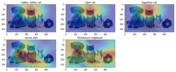
As you see it, the attention is highlighted over the cat whether it's tabby, tiger, or egyptian.
Apply CAM to MRNet network
Now comes the fun part: let's apply what we just did on the MRNet network we trained in the previous post to highlight the regions that activate most when the network detects an ACL tear.
There is however a subtle difference: MRNet's input is a set of MRI slices: CAMs will therefore get computed independently over each one. This results in a small modification of the returnCAM function.
For simplicity, we'll consider the network trained on sagittal plane (where ACL tear is best detected) only.
import sys
sys.path.append('../../mrnet')

import torch
import model
from dataloader import MRDataset
from tqdm import tqdm_notebook

task = 'acl'
plane = 'sagittal'
prefix = 'v3'

model_name = [name  for name in os.listdir('../models/')
              if (task in name) and
                 (plane in name) and
                 (prefix in name)][0]

is_cuda = torch.cuda.is_available()
device = torch.device("cuda" if is_cuda else "cpu")

mrnet = torch.load(f'../models/{model_name}')
mrnet = mrnet.to(device)

_ = mrnet.eval()

dataset = MRDataset('../data/',
                    task,
                    plane,
                    transform=None,
                    train=False)
loader = torch.utils.data.DataLoader(dataset,
                                     batch_size=1,
                                     shuffle=False,
                                     num_workers=0,
                                     drop_last=False)

def returnCAM(feature_conv, weight_softmax, class_idx):
    size_upsample = (256, 256)
    bz, nc, h, w = feature_conv.shape
    slice_cams = []
    for s in range(bz):
        for idx in class_idx:
            cam = weight_softmax[idx].dot(feature_conv[s].reshape((nc, h*w)))
            cam = cam.reshape(h, w)
            cam = cam - np.min(cam)
            cam_img = cam / np.max(cam)
            cam_img = np.uint8(255 * cam_img)
            slice_cams.append(cv2.resize(cam_img, size_upsample))
    return slice_cams
We create a list of patients who are subject to ACL tear to test CAM:
patients = []

for i, (image, label, _) in tqdm_notebook(enumerate(loader), total=len(loader)):
    patient_data = {}
    patient_data['mri'] = image
    patient_data['label'] = label[0][0][1].item()
    patient_data['id'] = '0' * (4 - len(str(i))) + str(i)
    patients.append(patient_data)

acl = list(filter(lambda d: d['label'] == 1, patients))
For each patient in the acl list, we generate a set of CAMs for each of the MRI slices and then we save everything on disk.
def create_patiens_cam(case, plane):
    patient_id = case['id']
    mri = case['mri']

    folder_path = f'./CAMS/{plane}/{patient_id}/'
    if os.path.isdir(folder_path):
        shutil.rmtree(folder_path)
    os.makedirs(folder_path)
    os.makedirs(folder_path + 'slices/')
    os.makedirs(folder_path + 'cams/')

    params = list(mrnet.parameters())
    weight_softmax = np.squeeze(params[-2].cpu().data.numpy())

    num_slices = mri.shape[1]
    global feature_blobs
    feature_blobs = []
    mri = mri.to(device)
    logit = mrnet(mri)
    size_upsample = (256, 256)
    feature_conv = feature_blobs[0]

    h_x = F.softmax(logit, dim=1).data.squeeze(0)
    probs, idx = h_x.sort(0, True)
    probs = probs.cpu().numpy()
    idx = idx.cpu().numpy()
    slice_cams = returnCAM(feature_blobs[-1], weight_softmax, idx[:1])

    for s in tqdm_notebook(range(num_slices), leave=False):
        slice_pil = (transforms
                     .ToPILImage()(mri.cpu()[0][s] / 255))
        slice_pil.save(folder_path + f'slices/{s}.png',
                       dpi=(300, 300))

        img = mri[0][s].cpu().numpy()
        img = img.transpose(1, 2, 0)
        heatmap = (cv2
                    .cvtColor(cv2.applyColorMap(
                        cv2.resize(slice_cams[s], (256, 256)),
                        cv2.COLORMAP_JET),
                               cv2.COLOR_BGR2RGB)
                  )
        result = heatmap * 0.3 + img * 0.5

        pil_img_cam = Image.fromarray(np.uint8(result))
        pil_img_cam.save(folder_path + f'cams/{s}.png', dpi=(300, 300))
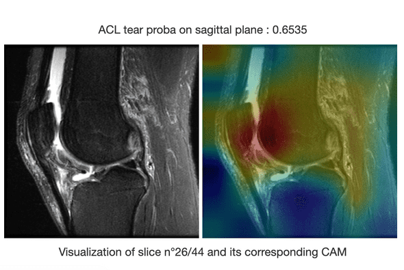
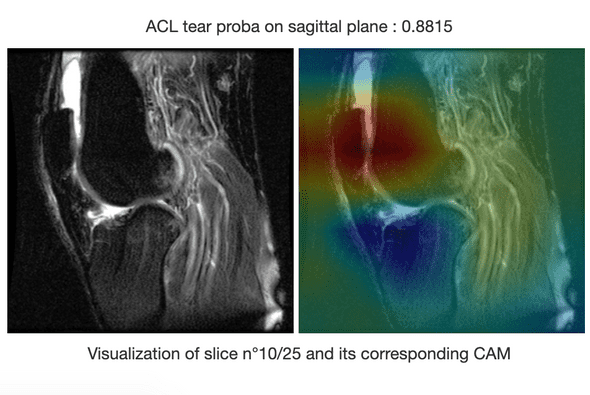
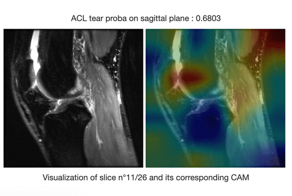
Some examples of highlighted ACL tears
Here are some examples of CAMs that spot knee injuries on MRI slices.
Conclusion
In this post we learnt about Class Activation Map which is an interpretability technique applied to convnets that have a global average pooling layer. We learnt how to implement it in PyTorch and apply it to a real medical application: highlighting knee injuries from MRI slices.
In order to go further and allow easier exploration of the MRNet data and the CAMs, I put in place a dash application that allows to visualize for a given patient, the CAMs over the 3 MRI (axial, sagittal and coronal) and through all the slices. This will allow to quickly switch from a patient to another to spot injuries.
If you're interested in running the application, the code is available on github repo under the folder dash. I won't unfortunately go into much details about it here, but if you're facing a problem running it, you can open an issue.
Here's a quick video demo of the dash application: